Contact mechanics

Contact models turn a calibrated force-indentation segment into parameters such as reduced or sample modulus. They are conditional physical models, not generic curve shapes: geometry, elasticity, adhesion, substrate effects, contact-point choice, and fit depth all determine whether a fitted number is meaningful.

SPM-Kit implements spherical/paraboloidal and conical elastic laws. The geometry parameters are measured inputs, not fit decorations.

Reduced modulus

For sample modulus \(E_s\) (Pa), sample Poisson ratio \(\nu_s\), tip modulus \(E_t\) (Pa), and tip Poisson ratio \(\nu_t\),

\[ \frac{1}{E^*}=\frac{1-\nu_s^2}{E_s}+\frac{1-\nu_t^2}{E_t}. \]

\(E^*\) is the reduced modulus (Pa). SPM-Kit's main elastic fitter assumes a rigid tip, so \(E_s=E^*(1-\nu_s^2)\). This approximation fails when tip compliance is not negligible.

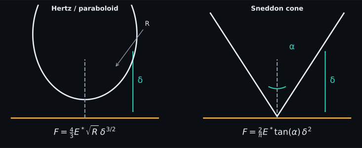
Hertz sphere and paraboloid

\[ F=\frac{4}{3}E^*\sqrt{R}\,\delta^{3/2}. \]

\(F\) is normal load (N), \(R\) tip radius (m), and \(\delta\) indentation (m). Assumptions include small-strain elastic, frictionless, non-adhesive contact between smooth bodies; an isotropic homogeneous half-space; and contact radius small relative to sample thickness and relevant curvature. In spmkit.core.analysis.mechanics.fit_hertz, sphere and paraboloid use this same local law. Current evidence is LEVEL 2 — NUMERICALLY_VERIFIED for the declared synthetic-recovery cases, not physical validation.

Sneddon cone

\[ F=\frac{2}{\pi}E^*\tan(\alpha)\,\delta^2. \]

\(\alpha\) is cone half-angle (rad). The other symbols and units are as above. The ideal cone is singular at its apex, so a real rounded tip may behave spherically at shallow indentation and conically only over a later interval. mechanics.fit_hertz(..., model="cone", half_angle=...) implements this law. It has synthetic recovery evidence at LEVEL 2 within the tested interval.

DMT offset path

The implemented DMT path uses a spherical elastic term plus a constant adhesive offset:

\[ F=\frac{4}{3}E^*\sqrt{R}\,\delta^{3/2}-F_{\mathrm{adh}}. \]

\(F_{\mathrm{adh}}\) is the measured pull-off magnitude (N). This is a specific operational approximation in mechanics.fit_hertz(..., model="dmt"), suitable for testing the declared offset model. It is not a complete material-selection rule for the DMT adhesion regime. Synthetic modulus/adhesion recovery supports LEVEL 2; no physical-reference campaign promotes it further.

Experimental JKR

SPM-Kit's experimental JKR route uses contact radius \(a\) (m), work of adhesion \(w\) (J m\(^{-2}\)), radius \(R\) (m), and reduced modulus \(E^*\) (Pa):

\[ \delta(a)=\frac{a^2}{R}-\sqrt{\frac{2\pi w a}{E^*}}, \qquad F(a)=\frac{4E^*a^3}{3R}-\sqrt{8\pi wE^*a^3}. \]

spmkit.core.analysis.experimental.fit_jkr performs a bounded grid search and is explicitly marked experimental. Analytical construction and synthetic recovery support a narrow LEVEL 2 numerical claim, including the \(w\to0\) Hertz limit. They do not validate JKR for a particular material or tip.

Fit-window discipline

• Exclude non-contact points and pull-off unless the selected model includes them.
• Keep indentation small enough for the assumed geometry, but large enough to exceed contact-point and noise uncertainty.
• Repeat fits across plausible contact points and windows.
• Inspect residual structure, \(R^2\), RMSE, point count, and parameter stability.
• Treat substrate, viscoelasticity, plasticity, poroelasticity, roughness, and adhesion regime as model-selection questions, not nuisance noise.

In automation, use spmkit forcecurve; for maps use spmkit forcemap. Fathom's Curva de fuerza and Mapa perspectives expose these paths. A modulus map inherits every calibration and model assumption of every pixel fit.

Force-distance curves · KPFM