Force-distance curves

A force-distance experiment parks the lateral position and drives the sample or tip along the vertical axis. The measured deflection signal becomes a force only after sensitivity and cantilever-stiffness calibration; the commanded scanner position becomes indentation only after contact and cantilever bending are accounted for.

Idealized force-distance regions. Real sign and axis directions depend on the instrument export, so SPM-Kit normalizes them before display and fitting.

From detector signal to force

For a detector signal \(V\) in volts, a deflection sensitivity \(S\) in metres per volt, and cantilever stiffness \(k\) in newtons per metre,

\[ d = S(V-V_0), \qquad F = k d. \]

\(d\) is cantilever deflection (m), \(V_0\) is the non-contact baseline (V), and \(F\) is normal force (N). This linear conversion assumes the detector response and cantilever remain in their calibrated regimes. A wrong sensitivity or \(k\) scales every subsequent force and modulus result.

If \(z\) is the imposed vertical displacement and \(z_c\) the contact position, a common indentation convention is

\[ \delta=(z-z_c)-d, \]

where indentation \(\delta\) is in metres. Axis orientation can reverse the first term; the implemented reader/curve convention governs, not the visual direction of a vendor plot.

Approach and retract

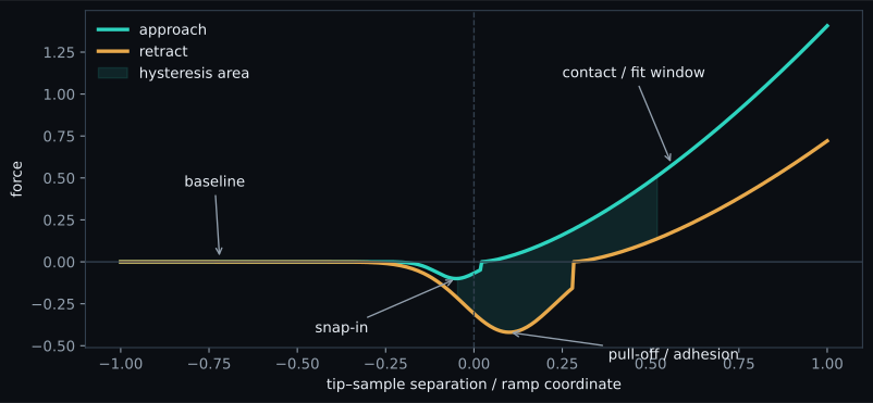
1. Baseline: far from the surface, fit and subtract offset or drift without including interaction points.
2. Snap-in: an attractive force gradient can exceed the cantilever restoring gradient, producing a sudden transition to contact.
3. Contact and loading: force rises as the tip indents the sample and bends the cantilever. This is the candidate fit region for a contact model.
4. Retract: adhesion can hold the tip after the drive reverses.
5. Pull-off: the most negative corrected force is an operational adhesion magnitude under the declared sign convention.
6. Hysteresis: the area between compatible approach and retract paths has units of joules and can represent dissipated work, but only after sampling, speed, baseline, and branch alignment are controlled.

Segmentation is part of the measurement

Contact-point error changes both the origin and the fitted indentation range. SPM-Kit provides threshold and ratio-of-variances paths, and the force pipeline can use a joint contact fit. None removes the need to inspect the result.

Common failure modes include baseline curvature, hydrodynamic drag, optical interference, detector saturation, piezo creep, a double contact, plasticity, tip contamination, insufficient non-contact data, and fitting through pull-off. Flat residuals and a high \(R^2\) do not prove the physical model is appropriate.

SPM-Kit path

spmkit.core.analysis.forcecurve handles display-axis normalization and the public curve fit. spmkit.core.pipeline.force_ops applies calibration, contact detection, and model fitting to typed ForceCurve objects. The direct command is:

spmkit forcecurve measurement.jpk-force --curve 0 --model sphere --tip-radius 1e-8

Fathom exposes a single curve in Curva de fuerza (force) and force-volume property maps in Mapa (map). The calibration source, contact method, model, tip geometry, Poisson ratio, and retained fit interval belong in provenance.

Evidence boundary

Claim	Current support	Boundary
calibrated signal conversion and curve orchestration	software tests	does not certify an instrument calibration
contact detection and elastic fits	synthetic numerical recovery	does not establish a universal contact point on experimental curves
force-volume property maps	scalar/vectorized consistency and synthetic recovery	the two internal routes are not independent external references
adhesion and hysteresis interpretation	implemented observables	no broad public physical-reference campaign

Operating modes · Contact mechanics