Resonance and mass sensing

A cantilever mode can be approximated as a damped harmonic oscillator. That model connects resonance frequency to stiffness and modal mass, but quantitative mass sensing also depends on mode shape, load position, added-mass distribution, fluid damping, temperature, detector calibration, and the definition of the bare state.

Added mass lowers the idealized resonance. Peak shape and width carry damping information; a real spectrum can contain backgrounds and multiple modes.

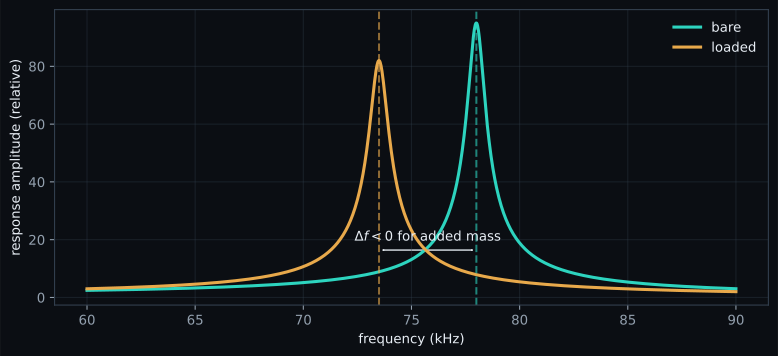
Oscillator and quality factor

For stiffness \(k\) (N m\(^{-1}\)) and effective modal mass \(m_{\mathrm{eff}}\) (kg),

\[ f_0=\frac{1}{2\pi}\sqrt{\frac{k}{m_{\mathrm{eff}}}}, \qquad m_{\mathrm{eff}}=\frac{k}{(2\pi f_0)^2}. \]

\(f_0\) is in hertz. For a narrow single resonance, the operational bandwidth relation is

\[ Q=\frac{f_0}{\Delta f_{\mathrm{FWHM}}}, \]

where \(Q\) is dimensionless and \(\Delta f_{\mathrm{FWHM}}\) is the full width at half maximum (Hz) under the selected amplitude/power convention.

resonance.find_resonance uses the peak and half-height width. resonance.fit_sho fits an amplitude-spectral-density SHO model with a noise floor when SciPy is available and otherwise returns the peak-based estimate.

Thermal noise and stiffness

Ideal equipartition gives

\[ \tfrac12 k\langle x^2\rangle=\tfrac12 k_B T. \]

\(x\) is calibrated deflection (m), \(\langle x^2\rangle\) its variance (m\(^2\)), \(k_B\) the Boltzmann constant (J K\(^{-1}\)), and \(T\) temperature (K). SPM-Kit implements

\[ k=\chi\frac{k_BT}{\langle x^2\rangle}, \]

with a configurable mode/detection correction \(\chi\) and default 0.817 in core.analysis.calibration.spring_constant_thermal. This requires a calibrated deflection spectrum with noise-background treatment. The Sader method is explicitly not implemented.

Effective and added mass

For a load treated at position \(x/L\) along a cantilever, the implemented position correction is

\[ k(x)=\frac{k(L)}{(x/L)^3}. \]

With bare frequency \(f_b\) and loaded frequency \(f\),

\[ \Delta m=\frac{k(x)}{4\pi^2} \left(\frac{1}{f^2}-\frac{1}{f_b^2}\right). \]

\(\Delta m\) is in kilograms. The relation assumes the one-mode lumped model and the declared load-position correction. Distributed loads, shape changes, stiffness changes, or fluid-property changes can shift frequency without representing only added mass.

Evaporation and the d² diagnostic

For a spherical droplet of density \(\rho\) (kg m\(^{-3}\)), SPM-Kit converts positive added mass to radius \(r\) (m) with

\[ r=\left(\frac{3\Delta m}{4\pi\rho}\right)^{1/3}. \]

It then fits the diffusion-limited diagnostic

\[ d^2(t)=d_0^2-Kt,\qquad d=2r, \]

where \(K\) has units m\(^2\) s\(^{-1}\). fit_d2_law labels a fit is_diffusion_limited when $R^2>0.95`; that boolean is an implementation criterion, not proof that all physical assumptions hold.

Measurement path versus educational simulation

extract_thermal and load_evaporation_series read NanoSurf thermal-tuning metadata and spectra; spmkit evaporation FOLDER builds the time series; Fathom uses Sintonía térmica (resonance) and Evaporación (evaporation). core.analysis.simulation separately generates idealized thermal spectra and mass-loaded shifts for Simulador. Simulation demonstrates equations; it is not a calibration reference.

The current scientific-status classification is LEVEL 1 — SOFTWARE_VERIFIED for SHO, thermal-calibration, and mass-sensing utilities. Unit tests and controlled numerical cases exercise these paths, while selected experimental files provide development context. There is no frozen public calibrated physical-reference campaign, no general nanogram-resolution claim, and no basis for the legacy statement that a particular real instrument was recovered to a universal percentage.

Spectral analysis · Implementation map